Will Gagne-Maynard by wgagne-maynard

Working with the IPUMSR package

It’s been a while since I last posted. In the meantime, I’ve got a new job at IHME, working on the geospatial team. I’ve been working a lot with R, specifically using it to clean + process large survey datasets.

Recently there was a new package released to work with IPUMS data in R, IPUMSR.

I thought I would try to play around with it and see what interesting data I can find, as I haven’t had much exposure to IPUMS data yet.

First step, install some packages, including ipumsr.

Earlier, I downloaded some NHGIS data from the IPUMS website. This process was not exactly painless, as there’s a lot of data available and it makes it slightly clumsy to grab what you’re looking for.

In the end, I downloaded data from the 2010 census at the census block level, along with the linked shapefiles.

Right now I’m just going to see what I can find in the data on vacancy rates + non-relative households.

## Set paths to the tables and shapefiles
nhgis_csv <- "C:/Users/gagnemaw/Desktop/nhgis0005_csv.zip"
nhgis_shp <- "C:/Users/gagnemaw/Desktop/nhgis0005_shape.zip"

This is where the ipumsr package comes in handy. The package contains a variety of functions to help read the IPUMS data into R. There are options to read microdata( read_ipums_micro), to read the metadata(read_ipums_ddi()) and functions to read in NHGIS data, which I’m using below. This allows for an easy way to load in both the survey data and attached shapefiles for plotting + analysis.

Right now I’m just looking at vacancy rates per census block.

I made a new variable, vacant_perc, for the % of vacant housing within a census block and subset to King County for simplified mapping / interpretation.

nhgis <- nhgis %>% mutate(vacant_perc = IFE003 / IFE001 * 100)

nhgis_subset <- nhgis %>% 
  filter(COUNTY %in% c("King County"))

Now on to plotting! The development version of ggplot2 has a new geom_sf() function that makes it incredbly easy to make maps. If needed, update ggplot via devtools::install_github(“tidyverse/ggplot2”).

if ("geom_sf" %in% getNamespaceExports("ggplot2")) {
  ggplot(data = nhgis_subset, aes(fill = vacant_perc)) +
    geom_sf(linetype="blank")
    
  }

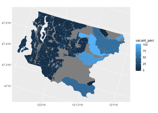
Mapping all of King Country really just shows the larger census blocks out east. Let’s try to figure out how to focus on just the Seattle area.

One simple way is just to use congressional districts. I mapped district 7 (Seattle, WA + Vashon Island), represented by Pramila Jayapal.

An important addition here is the linetype = "blank" argmument that I cribbed from the ipumsr vignette. This doesn’t plot the outlines for the shapefiles, so we can actually see some of the detail in the smaller census blocks.

nhgis_07 <- nhgis_subset[nhgis_subset$CDA == "07",]

if ("geom_sf" %in% getNamespaceExports("ggplot2")) {
  ggplot(data = nhgis_07, aes(fill = vacant_perc, colour=vacant_perc)) +
    geom_sf(linetype = "blank") + 
    coord_sf(crs =st_crs(3395))
    
  }

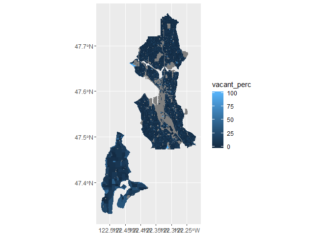Now I have a map, but the area is still too large to get a clear picture of any spatial trends.

Option 1. Look at an even smaller area.

Option 2. Aggregate up to a greater spatial extent.

Option 1 is easier, so I’m starting with that. I’m further subsetting the data on state legislative districts, focusing on districts 36,43 and 46 in North Seattle.

nhgis_leg <- nhgis_07[nhgis_07$SLDUA %in% c("036","043","046"),]
if ("geom_sf" %in% getNamespaceExports("ggplot2")) {
  ggplot(data = nhgis_leg, aes(fill = vacant_perc)) +
    geom_sf(linetype = "blank") + 
    ##manually set limits to show variation in blocks with lower vacancy rates
    scale_fill_gradient(limits=c(0,20)) + 
        coord_sf(crs =st_crs(3395))

    
  }

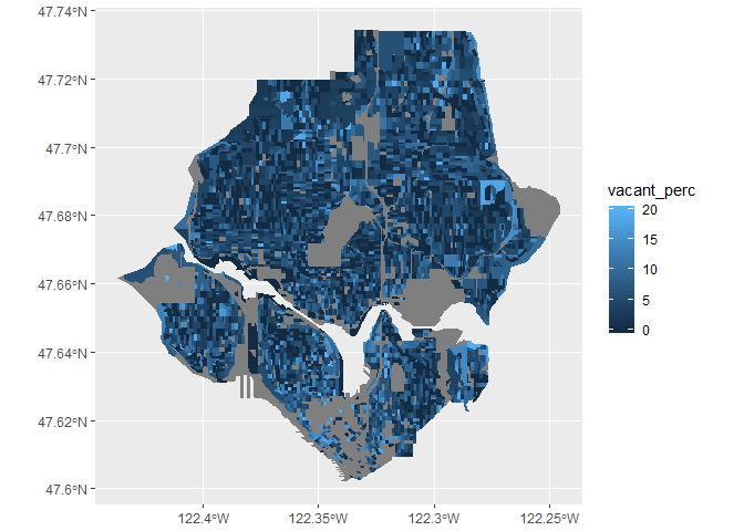
Looks good! No immediate trends in vacancy rates, although 20% vacancy seems high for certain blocks in 2010 Seattle. I need to look more into how these are actually measured.

Now that I have a hang of importing and plotting data, I want to take a shot at some other datasets available from the NHGIS systmem. Using the same 2010 census, I thought I’d take a look at the # of households with non-relatives. This looks like it might be a useful proxy for rentals or non single-family units.

##Create new variable for same legislative districts as above
nhgis_leg_2 <- nhgis_2_king[nhgis_2_king$SLDUA %in% c("036","043","046"),]
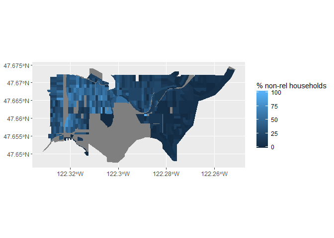
  ggplot(data = nhgis_leg_2, aes(fill = nonrel_household_per)) +
    geom_sf(linetype = "blank") + 
    labs(fill = "% non-rel households") + 
    ##manually set limits to show variation
    scale_fill_gradient(limits=c(0,50)) + 
        coord_sf(crs =st_crs(3395))

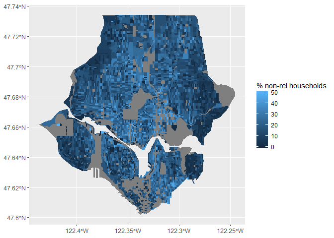
Some interesting trends jump out here. The area with the highest non-relative household % looks to be in the U-District, which would be expected due to the relatively high student population.

The areas of Magnolia, Madison Park and Laurelhurst all appear to have uniformly low percentages of non-relative households, which isn’t surprising given the largely single-family zoning of these neighborhoods.

This is most strikingly seen if we look at zipcode 98105, which includes both the U-District and Laurelhurst

nhgis_98105 <- nhgis_2_king[nhgis_2_king$ZCTA5A %in% c("98105"),]
  ggplot(data = nhgis_98105, aes(fill = nonrel_household_per)) +
    geom_sf(linetype = "blank") + 
    labs(fill = "% non-rel households") + 
    ##manually set limits to show variation
    scale_fill_gradient(limits=c(0,100)) + 
        coord_sf(crs =st_crs(3395)) 

Anyways, quick fun way to get to play with the IPUMSR package and get a handle on the data available on the NHGIS portal.

Now that I have a basic framework for working and plotting the data, I can ask more interesting questions. As a 20-something year old renter in Seattle who has lived next to a number of vacant properties, these were the fields that immediately popped out. Would be very interesting to see how these trends evolved over time, or if other census questions follow these geographic trends.